If you were a dishonest person, you could open up Mickwalker Ranch and get $20 million in government funding

You are using an out of date browser. It may not display this or other websites correctly.
You should upgrade or use an alternative browser.
You should upgrade or use an alternative browser.
Skinwalker Ranch S4 E11 Claims of "Wormhole" from LIDAR Scan with Gap
- Thread starter LeastWeasel
- Start date
NorCal Dave
Senior Member.
Yeah, but everybody has to wear tourist sandals and funny T shirts.If you were a dishonest person, you could open up Mickwalker Ranch and get $20 million in government funding
") To be fair, it was pretty warm in NorCal this weekend.
To be fair, it was pretty warm in NorCal this weekend.It's puzzling. Apparently Taylor was a lot more skeptical before he went to work on the show. He's not an idiot, but seems to rush towards conclusions without checking all his assumptions or data. He also has a tendency to roll out physics buzzwords ("Fraunhofer diffraction" being a favorite)
Yes, but this has been his schtick since the late '90s. When looking into Art's Parts I found the claim from Linda M. Howe that Taylor heard her on the radio and offered to help out:
https://www.metabunk.org/threads/meta-materials-from-ufos.12995External Quote:
However, there is a video from '04 with Linda Howe giving a presentation about the material in question. It's a bit of a slog, but I tried to queue it up (42:56) below where she talks about asking for help on the radio, presumably on Bell's Coast to Coast AM and gets response from an engineer and physicist from Huntsville AL named Travis Taylor that offers to help her. She then plays an audio recording of him and then shows some clips from the experiment. It looks like the 4:20 timestamp in the above quote where the sample jumps around and moves. She also claims the experiment took place in 1996:
Source: https://youtu.be/pfLUAiTnlcw?t=2576
And he was telling tale tales or at least making wild suggestions as soon as he got in with the UFO crowd:
http://www.ufowatchdog.com/howeufodebris.htmExternal Quote:Claims were made by a Tesla coil enthusiast in Alabama that the portion of the artifact in his possession acted strangely and tried to levitate in the presence of the electrostatic field of a Van de Graaf generator and a radio frequency source. We did perform a separate replication here, and found that our metal fragment danced about as well in the field of a Van de Graaf. And so did a piece of aluminum foil! Please understand that just about any small unattached mass will dance in the field of a 200,000 volt source! The mythos grew…
Note also, in LMH's description of the tests Taylor did with the magnesium/bismuth piece, it moved but a piece of aluminum did not. That's contradictory to the above paragraph that states aluminum foil moved around just like the MgBi piece when sufficient voltage was applied. Was LMH being shown what she wanted to see?
External Quote:
- 4:00 More electrode, moves a little.
- 4:20 Bis/Mag moves by itself in considerable sideways motion and falls off insulator cap. (637K Executable File)
- 4:29 Aluminum on insulator - no movement at all.
- 5:07 Bis/Mag with black bismuth side up. Nothing much happens.
- 5:20 Travis flips piece over so silver magnesium is on top - then there is more sideways motion when his finger enters the field. (601K Executable File)
- 6:20 Aluminum piece back on insulator cap; Travis using finger. But aluminum does not move around like bis/mag.
- 6:50 Travis summary.
- 8:30 END.
By the later '00s he was appearing in regularly in Ancient Aliens, hardly a science-based show, along with The UnXplained, Curse of Oak Island and other equally non-scientific bits of "reality TV":
https://en.wikipedia.org/wiki/Travis_S._Taylor
Seems like playing the "Legit Scientist With Supernatural Theories" character is something he's been aiming for going back 20+ years.
Mendel
Senior Member.
That's because Mick's focus is on doing science, not on "looking like a scientist".Yeah, but everybody has to wear tourist sandals and funny T shirts.
That's not a funny T shirt! That's funny shorts! Is it just me or did Einstein's legs look "athletic?"That's because Mick's focus is on doing science, not on "looking like a scientist".
Ann K
Senior Member.
Thats also an opera by Philip Glass:That's because Mick's focus is on doing science, not on "looking like a scientist".
Source: https://www.youtube.com/watch?v=a8kgAkTS7oM
NoParty
Senior Member.
This restores my faith in the promise of the internet (that social media was erasing). Thanks Mick!
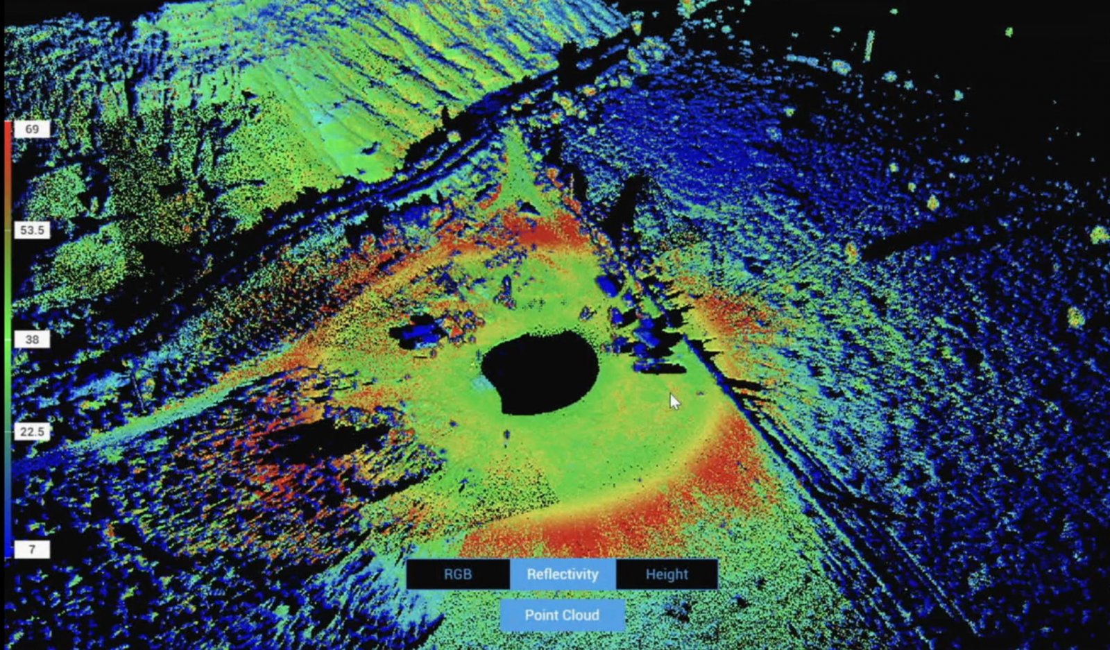
The black void has a very reasonable explanation, but what about that yellow and red ring?
This is a good point. If there was some distortion of the lidar there would also be a ring-like artifact in the visible (RGB Space) image. Here's the comparison again:From the image comparison (awesome website feature) I am more impressed by the lack of the red ring being expressed in RGB space rather than black blob size.
Note zero distortion in the visible image. So it's not bending light. So the ring is an artifact of the LIDAR system itself.
But what artifact? We know the drone isn't moving much (from the shadows) which means that for all points on the yellow ring there are two constants - the angle of incidence and the distance.
The yellow ring is about 35m from the center, the drone is about 10m above ground, so the line of sight distance from the drone to the yellow is about 36m (really still "about" 35m, with these rough guess).
My initial thought was angle of incidence - like there was a certain angle (atan(10/35) = 16°) at which there was maximum reflectivity dues to the geometry of the dust/sand. I thought that reflectivity would surely just decrease with distance.
Then I saw this:
https://www.mdpi.com/2072-4292/12/17/2855
View attachment 60530
These are two graphs of LIDAR intensity at varying incidence angles and ranges. While not specifically over dirt, we see a gradual decrease with increasing incidence angle. More importantly we see that reflectivity initially increases with distance (range), and then drops off.
Article: We can see that the intensity at each laser wavelength of the measured targets increases more rapidly at a distance from 4 to 8 m and then decreases less rapidly greater than that. When the measured range is shorter than around 8 m, the instrumental properties, such as the near-distance reducer or the refractor telescope's defocusing effect, have a significant influence on the raw intensities, and this makes the intensities disaccord with the radar range equation
Now this seems quite promising for ring creation, especially at the effect is more pronounced at longer wavelengths. The 8m vs. 35 m is an issue, but sensors differ. The DJI Zenmuse L1 is designed to fly at 50-100m
Last edited:
It looks more pronounced at shorter wavelengths to me. The lowest peaks in the graph are the 800+ nm and the 540 nm one (probably funky quantum physics going on). Extrapolating from the 800+ nm ones, the 905 nm wavelength that was used may go down to 5 in intensity, though the data aren't linear so the guess can be way off.especially at the effect is more pronounced at longer wavelengths
The reflectivity measured at the circle seems to be less than double than the closest point, judgind by the legend, so a smaller peak in intensity should be a better fit, I think.
Yeah, that's a bit odd. I misread the small diagram.It looks more pronounced at shorter wavelengths to me. The lowest peaks in the graph are the 800+ nm and the 540 nm one (probably funky quantum physics going on). Extrapolating from the 800+ nm ones, the 905 nm wavelength that was used may go down to 5 in intensity, though the data aren't linear so the guess can be way off.
Not the easiest thing to read, but yes, it seems the effect peaks at 653nm, but the order seems weird. There's another for a leaf, where it's quite different.
Mendel
Senior Member.
They all are of leaves.Not the easiest thing to read, but yes, it seems the effect peaks at 653nm, but the order seems weird. There's another for a leaf, where it's quite different.
Article: The backscatter intensity of the continuous light source was recorded at twenty laser wavelength channels (540~849 nm) for various samples. Leaf samples were collected from six common broadleaf plant species (Table 1), including Ficus elastica, Epipremnum aureum, Aglaonema modestum, Hibiscus rosa-sinensis Linn, Spathiphyllum kochii and Kalanchoe blossfeldiana Poelln.

The backscatter intensity per frequency would depend on the intensity of the laser and the color of the object, so I wouldn't read too much into it—that's not what the study was set up for.
jarlrmai
Senior Member.
LIDAR is used for so many things, ITD is one of them
https://www.fs.usda.gov/research/treesearch/59063LiDAR individual tree detection (ITD) is a promising tool for measuring forests at a scale that is meaningful ecologically and useful for forest managers.
I am thinking the artifact may have to do with the laser focus.But what artifact? We know the drone isn't moving much (from the shadows) which means that for all points on the yellow ring there are two constants - the angle of incidence and the distance.
The yellow ring is about 35m from the center, the drone is about 10m above ground, so the line of sight distance from the drone to the yellow is about 36m (really still "about" 35m, with these rough guess).
My initial thought was angle of incidence - like there was a certain angle (atan(10/35) = 16°) at which there was maximum reflectivity dues to the geometry of the dust/sand. I thought that reflectivity would surely just decrease with distance.
Then I saw this:
https://www.mdpi.com/2072-4292/12/17/2855
View attachment 60530
These are two graphs of LIDAR intensity at varying incidence angles and ranges. While not specifically over dirt, we see a gradual decrease with increasing incidence angle. More importantly we see that reflectivity initially increases with distance (range), and then drops off.
Article: We can see that the intensity at each laser wavelength of the measured targets increases more rapidly at a distance from 4 to 8 m and then decreases less rapidly greater than that. When the measured range is shorter than around 8 m, the instrumental properties, such as the near-distance reducer or the refractor telescope's defocusing effect, have a significant influence on the raw intensities, and this makes the intensities disaccord with the radar range equation
Now this seems quite promising for ring creation, especially at the effect is more pronounced at longer wavelengths. The 8m vs. 35 m is an issue, but sensors differ. The DJI Zenmuse L1 is designed to fly at 50-100m
https://www.edmundoptics.es/knowledge-center/application-notes/lasers/gaussian-beam-propagation/
The laser beam focuses at a certain point to a miniumm size (here called "waist"), for certain distance (here called "Rayleigh Range") where the intensity density (W/cm^2) maximizes, and then just diverges (very narrowly) around that maximum focus. but I'm not sure there are data of the system enough to calculate that distance from the laser source to the minimum waist point and see if it matches the distance.External Quote:
IIn many laser optics applications, the laser beam is assumed to be Gaussian with an irradiance profile that follows an ideal Gaussian distribution. All actual laser beams will have some deviation from ideal Gaussian behavior. The M2 factor, also known as the beam quality factor, compares the performance of a real laser beam with that of a diffraction-limited Gaussian beam.1 Gaussian irradiance profiles are symmetric around the center of the beam and decrease as the distance from the center of the beam perpendicular to the direction of propagation increases (Figure 1).
(...)
In Equation 1, I0 is the peak irradiance at the center of the beam, r is the radial distance away from the axis, w(z) is the radius of the laser beam where the irradiance is 1/e2 (13.5%) of I0, z is the distance propagated from the plane where the wavefront is flat, and P is the total power of the beam.
 of its maximum value")
Figure 1: The waist of a Gaussian beam is defined as the location where the irradiance is 1/e2 (13.5%) of its maximum value
However, this irradiance profile does not stay constant as the beam propagates through space, hence the dependence of w(z) on z. Due to diffraction, a Gaussian beam will converge and diverge from an area called the beam waist (w0), which is where the beam diameter reaches a minimum value. The beam converges and diverges equally on both sides of the beam waist by the divergence angle θ (Figure 2). The beam waist and divergence angle are both measured from the axis and their relationship can be seen in Equation 2 :
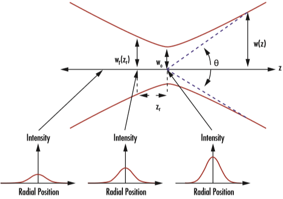
Figure 2: Gaussian beams are defined by their beam waist (w0), Rayleigh range (zR), and divergence angle (θ)
I believe the Rayleigh range can be calculated from divergence values of the laser, (which I guess may be known) so maybe one can compare that value to the width of the estimated "red ring" in the lidar images.
Edit to clarify: I do NOT mean the laser is out of focus. Maybe the word focus is not even correct. This is a phenomenon that appears in laser beams, that in a way I think it resembles focusing.
Last edited:
It may be that both effects presented by @Mick West and @jplaza are in effect and add up the waveforms. An issue is the fact that after the smooth gradient gets to red, it gets funky and there's no gradient for the falling side of the waveform. That's very likely a software issue, I think, but that's probably not something that can be easily proved without access to the drone and software that were used.
On the side, there's another evidence line for the ring being an artifact of the operation of the LIDAR system in the discontinuities where the angle from the ground was changed. I think the act of adjusting the viewing angle gave the software a few more data points to work with and get better results. The semicircles also don't quite connect. If you look closely, it's quite visible at the 7 o'clock discontinuity that the semicircle from the left side has a slightly smaller radius.
On the side, there's another evidence line for the ring being an artifact of the operation of the LIDAR system in the discontinuities where the angle from the ground was changed. I think the act of adjusting the viewing angle gave the software a few more data points to work with and get better results. The semicircles also don't quite connect. If you look closely, it's quite visible at the 7 o'clock discontinuity that the semicircle from the left side has a slightly smaller radius.
Ravi
Senior Member.
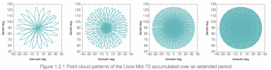
As it was found they seem to use the sensor as mentioned by @Beck in post #36, I looked into the manual of the sensor (Livox MID-70). They use a radial pattern scanning (non moving) method. The pattern the scanner makes, looks like a daisy wheel / Lissajous curve, covering the FoV.
This means the sensor makes, in 1.5 sec, scans of it's full FoV (which is 70.2 degrees circular). The scan area is thus cone shaped and the sensor and/or the drone has to rotate to move the sensor to a new fresh area to be scanned again. The scan of the full circle area as shown in the show means they need at least 360/70.2 = 5.1 x repositioning to make a gapless point cloud. Perhaps they used 6 positions, taking say 5 sec to rotate each time, which means a full 360 scan is finished in 6 x 1.5sec x 5 = ± 45sec.
Do they mention anything about this in the tv show?
https://terra-1-g.djicdn.com/65c028...d-70/new/Livox Mid-70 User Manual_EN_v1.2.pdfExternal Quote:

This means the sensor makes, in 1.5 sec, scans of it's full FoV (which is 70.2 degrees circular). The scan area is thus cone shaped and the sensor and/or the drone has to rotate to move the sensor to a new fresh area to be scanned again. The scan of the full circle area as shown in the show means they need at least 360/70.2 = 5.1 x repositioning to make a gapless point cloud. Perhaps they used 6 positions, taking say 5 sec to rotate each time, which means a full 360 scan is finished in 6 x 1.5sec x 5 = ± 45sec.
Do they mention anything about this in the tv show?
Attachments
Last edited:
Ann K
Senior Member.
It's at the area where bare dirt gives way to vegetation, so a different reflectivity.If you look closely, it's quite visible at the 7 o'clock discontinuity that the semicircle from the left side has a slightly smaller radius.
Ravi
Senior Member.
No problem, it gives food for thought!@Ravi I don't think that they rotated the drone too fast. Aside from shadows behind objects, there aren't other undefined areas.
I am thankful for your post, though. It answers a lot of what I've been trying to figure out today. Just what the doctor ordered .
BTW the red zone/cirlce may well be a (residual) calibration artefacts from the sensor system, but not sure.
Right, squinting isn't all that good. Zooming in to that portion made me lose sight of the forest for the trees, but the change in vegetation doesn't exactly match the red ring, either.I think @Ravi may have pointed out the way... If not documentation from the manufacturer, then community content may be relevant. This kind of spurious data ring may be a well known phenomenon amongst users of this particular LIDAR system.It's at the area where bare dirt gives way to vegetation, so a different reflectivity.
Last edited:
The manual results were a bit unsatisfying, so here's a programmatic explanation of how the black shape arises.
Python:
import matplotlib.pyplot as plt
import numpy as np
from matplotlib.patches import Circle

# Define the radii
rA = 85
rB_initial = 100
rB_final = 60

# Define the number of points to generate
num_points = 1000

# Define the reduction and increment angle in radians
angle_change = np.pi / 36

# Generate theta values
theta = np.linspace(0, 2*np.pi, num_points)

# Define the function for the radius of B
def rB(theta):
    if theta <= np.pi:
        return rB_initial
    elif theta <= np.pi + angle_change:
        # Decrease from 100 to 80
        return rB_initial - (rB_initial - rB_final) * (theta - np.pi) / angle_change
    elif theta <= 2*np.pi - angle_change:
        return rB_final
    else:
        # Increase from 80 to 100
        return rB_final + (rB_initial - rB_final) * (theta - (2*np.pi - angle_change)) / angle_change

# Generate the (x, y) coordinates for the path of circle A
xA = np.array([(rB(t) + rA) * np.cos(t) for t in theta])
yA = np.array([(rB(t) + rA) * np.sin(t) for t in theta])

# Create the plot
fig, ax = plt.subplots(figsize=(10, 10))
ax.plot(xA, yA, label='Path of Circle A')

# Show the path traced by Circle A using circles
for (x, y) in zip(xA[::2], yA[::2]):
    circle = Circle((x, y), rA, fill = False, edgecolor = 'r', linewidth = 0.5)
    ax.add_patch(circle)

ax.set_title('Path Covered by Circle A around Circle B with Gradually Reducing and then Increasing Radius')
ax.set_xlabel('X')
ax.set_ylabel('Y')
ax.set_aspect('equal', adjustable='box')
plt.legend()
plt.show()Similar but using an ellipse:

And the actual shape:

And the actual shape:
Python:
import matplotlib.pyplot as plt
import numpy as np
from matplotlib.patches import Ellipse

# Define the radii
rA_long = 80
rA_short = 40
rB_initial = 100
rB_final = 60

# Define the number of points to generate
num_points = 1000

# Define the reduction and increment angle in radians
angle_change = np.pi / 36

# Generate theta values
theta = np.linspace(0, 2*np.pi, num_points)

# Define the function for the radius of B
def rB(theta):
    if theta <= np.pi:
        return rB_initial
    elif theta <= np.pi + angle_change:
        # Decrease from 100 to 80
        return rB_initial - (rB_initial - rB_final) * (theta - np.pi) / angle_change
    elif theta <= 2*np.pi - angle_change:
        return rB_final
    else:
        # Increase from 80 to 100
        return rB_final + (rB_initial - rB_final) * (theta - (2*np.pi - angle_change)) / angle_change

# Generate the (x, y) coordinates for the path of the center of the ellipse
xA = np.array([(rB(t) + rA_long) * np.cos(t) for t in theta])
yA = np.array([(rB(t) + rA_long) * np.sin(t) for t in theta])

# Create the plot
fig, ax = plt.subplots(figsize=(10, 10))
ax.plot(xA, yA, label='Path of Center of Ellipse')

# Show the path traced by the Ellipse using ellipses
for (x, y, t) in zip(xA[::2], yA[::2], theta[::2]):
    ellipse = Ellipse((x, y), rA_long*2, rA_short*2, angle=np.degrees(t), fill = False, edgecolor = 'r', linewidth = 0.5)
    ax.add_patch(ellipse)

ax.set_title('Path Covered by Center of Ellipse around Circle B with Gradually Reducing and then Increasing Radius')
ax.set_xlabel('X')
ax.set_ylabel('Y')
ax.set_aspect('equal', adjustable='box')
plt.legend()
plt.show()Mendel
Senior Member.
That seems to explain the inner 'black hole' effect very well. I suspect that the 'ellipses' are much longer than this, however; the scanned area seems to extend a very long way, far outside the mysterious 'red' ring of greatest reflectance.
Article: 
The black boundaries of the colored regions are conic sections.
That said, qualitatively that's not going to change the "black hole" shape.
Eburacum
Senior Member.
Thanks for the diagram of conic sections.
However, I put 'ellipse' in quote marks because the scanning system of this particular LiDAR sensor uses a Lissajous curve, which is similar to, but not identical with, an ellipse. Each successive segment of the curve is slightly displaced from the one before, so that the entire field of view is eventually covered. My point is that these curves must be significantly more elongated in the radial direction than shown on Mick West's diagram, because they record data right to the edge of the map, and probably beyond that.
I'm still convinced that the red ring (and the yellow ring directly inside it) is an artifact of the sensor system, and it may simply be that the density of the overlapping curves reaches a maximum in that region.
Note as well that all the upstanding objects in that region are dark blue, suggesting that they return much less light to the sensor than the ground surface.
Mendel
Senior Member.
X-Y Lissajous curves:The pattern the scanner makes, looks like a daisy wheel / Lissajous curve, covering the FoV.
https://terra-1-g.djicdn.com/65c028...d-70/new/Livox Mid-70 User Manual_EN_v1.2.pdfExternal Quote:
The diagram that Ravi gave is distinct from a Lissajous curve. A Lissajous curve covers a rectangle eventually, while the Lidar diagram describes a cone centered on 90⁰ vertical and 0⁰ azimuth as the convex hull of the scanned space. This scan cone intersects the ground, and depending on the angle, the ground track of the scan cone is one of the conic sections (if the ground is approximately level). Note that the parabola and the hyperbola encompass infinite areas, which allow them to reach the edge of the map; these are obtained once the upper tangent of the scan cone no longer intersects the ground.However, I put 'ellipse' in quote marks because the scanning system of this particular LiDAR sensor uses a Lissajous curve, which is similar to, but not identical with, an ellipse. Each successive segment of the curve is slightly displaced from the one before, so that the entire field of view is eventually covered.
Note as well that all the upstanding objects in that region are dark blue, suggesting that they return much less light to the sensor than the ground surface.
Last edited:
Agent K
Senior Member
Leaves reflect Near IR.Leaves absorb IR while dirt does not.
https://www.metabunk.org/threads/co...ectrum-the-definitive-guide.10548/post-229407
Eburacum
Senior Member.
I imagine a gradual circular scan, using the MD70 scanner with a 70 degree field of view. This would create a ring-like pattern with a central hole, but also with a brighter region at the central part of the cone.
I can't replicate a smooth scan, but if you convert the MD70 circular scan into an ellipse, then replicate it six times in a circle (complete with central wormhole gap) you get a brighter ring (like this).

I can't replicate a smooth scan, but if you convert the MD70 circular scan into an ellipse, then replicate it six times in a circle (complete with central wormhole gap) you get a brighter ring (like this).
Agent K
Senior Member
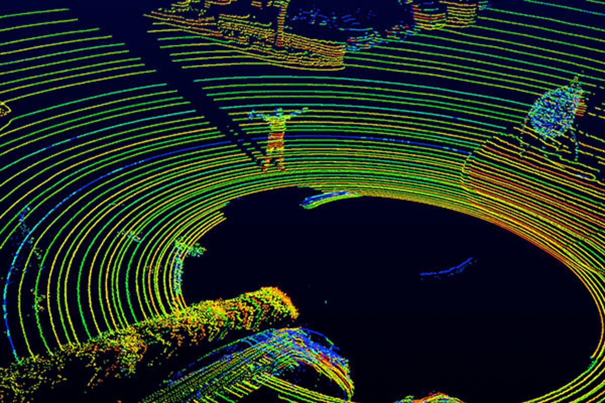
There's a hole in the center of every self-driving car with a Velodyne lidar.
https://newatlas.com/velodyne-lidar-vls-128-sensor/52453/.
https://newatlas.com/velodyne-lidar-vls-128-sensor/52453/.
Agent K
Senior Member
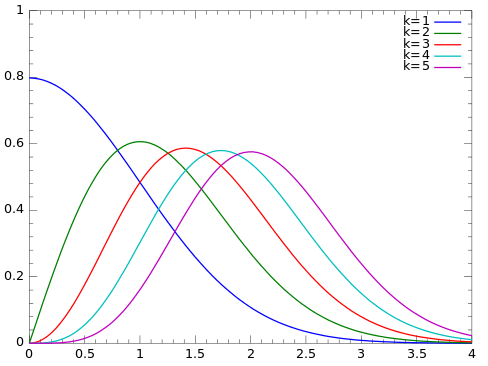
I don't think the following explains the ring artifact, but it reminded me of the fact that if you take a 2D Gaussian distribution, where the X and Y positions are Gaussian, then the distance from the center, sqrt(X^2+Y^2), follows the chi distribution with k=2. So even though the X and Y distributions are densest at the center, the distance from the center is the least dense at the center.I imagine a gradual circular scan, using the MD70 scanner with a 70 degree field of view. This would create a ring-like pattern with a central hole, but also with a brighter region at the central part of the cone.
I can't replicate a smooth scan, but if you convert the MD70 circular scan into an ellipse, then replicate it six times in a circle (complete with central wormhole gap) you get a brighter ring (like this).
https://en.wikipedia.org/wiki/Chi_distribution
Probability density function
Mendel
Senior Member.
I stand corrected.Leaves reflect Near IR.
https://science.nasa.gov/ems/08_nearinfraredwaves
https://www.sciencedirect.com/science/article/pii/S1110982317300327
I expect that to be cleared in the software, otherwise you'd get that artifact wherever you point the sensor and however you move the drone.I imagine a gradual circular scan, using the MD70 scanner with a 70 degree field of view. This would create a ring-like pattern with a central hole, but also with a brighter region at the central part of the cone.
I can't replicate a smooth scan, but if you convert the MD70 circular scan into an ellipse, then replicate it six times in a circle (complete with central wormhole gap) you get a brighter ring (like this).
View attachment 60568
Eburacum
Senior Member.
No, I don't think so. Generally, airborne LiDAR scans are performed by a moving aircraft that builds up a composite image from several different viewpoints; scanning from a single point can lead to data dropouts and other unwanted effects.
Mick West performed a sensible scan in his recreation - that involved moving the LiDAR scanner and sensor on his phone up and down the garden, eliminating both the black hole region with no data, and any other artifacts caused by the angle of the scan.

Mick West performed a sensible scan in his recreation - that involved moving the LiDAR scanner and sensor on his phone up and down the garden, eliminating both the black hole region with no data, and any other artifacts caused by the angle of the scan.
Last edited:
Eburacum
Senior Member.
I added another layer of daisy-wheel scans to the image, and the brighter ring still persists.

To make my intentions clear, I am using this particular image from the manual posted by @Ravi, which shows what the scanning pattern from this particular model looks like when scanning a surface from directly above.
(image posted by ravi)
-
-
To quote Ravi in that post
-
In my image I have assumed that they rotated the sensor 12 times, making a fairly dense point cloud except at the edges; this shows a ring-like brightening which corresponds with the red ring in the 'reflectivity' image. However it is very likely that they rotated the sensor (relatively) smoothly, which would produce something like the (relatively) smooth red ring seen in this image from the show.
Disclaimer; I can't replicate this smooth rotation myself using the graphic tools I have available, so the image above is my best attempt.
-
-
The only thing that now puzzles me is that this image is labelled 'reflectivity'. I think it actually represents 'data return intensity', which would be a different thing. Reflectivity, or albedo, would be derived by dividing the intensity of the emitted light by the intensity of the received light, and if so this ring-like phenomenon I believe I have detected would be largely, or wholly, eliminated.
To make my intentions clear, I am using this particular image from the manual posted by @Ravi, which shows what the scanning pattern from this particular model looks like when scanning a surface from directly above.
(image posted by ravi)
-
-
To quote Ravi in that post
-This means the sensor makes, in 1.5 sec, scans of it's full FoV (which is 70.2 degrees circular). The scan area is thus cone shaped and the sensor and/or the drone has to rotate to move the sensor to a new fresh area to be scanned again. The scan of the full circle area as shown in the show means they need at least 360/70.2 = 5.1 x repositioning to make a gapless point cloud. Perhaps they used 6 positions, taking say 5 sec to rotate each time, which means a full 360 scan is finished in 6 x 1.5sec x 5 = ± 45sec.
-
In my image I have assumed that they rotated the sensor 12 times, making a fairly dense point cloud except at the edges; this shows a ring-like brightening which corresponds with the red ring in the 'reflectivity' image. However it is very likely that they rotated the sensor (relatively) smoothly, which would produce something like the (relatively) smooth red ring seen in this image from the show.
Disclaimer; I can't replicate this smooth rotation myself using the graphic tools I have available, so the image above is my best attempt.
-
-
The only thing that now puzzles me is that this image is labelled 'reflectivity'. I think it actually represents 'data return intensity', which would be a different thing. Reflectivity, or albedo, would be derived by dividing the intensity of the emitted light by the intensity of the received light, and if so this ring-like phenomenon I believe I have detected would be largely, or wholly, eliminated.
Last edited:
Ravi
Senior Member.
@Eburacum
Not sure if I agree with your conclusion that a denser point cloud will show a higher "back reflection intensity". I am certain the calibration takes care of any system errors that one can expect. But even so, a denser point cloud is a cloud of individual measurements, thus I/O per pulse, where the amount of them does not influence the magnitude of intensity.
Not sure if I agree with your conclusion that a denser point cloud will show a higher "back reflection intensity". I am certain the calibration takes care of any system errors that one can expect. But even so, a denser point cloud is a cloud of individual measurements, thus I/O per pulse, where the amount of them does not influence the magnitude of intensity.
so this ring-like phenomenon I believe I have detected should be largely, or wholly, eliminated.
About halfway through the rotation, the viewing angle gets adjusted, but there is no shift in the radius of the corresponding reflexive semicircle, which doesn't match what your hypothesis predicts.
Just what I was thinking.But even so, a denser point cloud is a cloud of individual measurements, thus I/O per pulse, where the amount of them does not influence the magnitude of intensity.
Eburacum
Senior Member.
This may be merely subjective, but I think it does. Remember to ignore the dark shadows.About halfway through the rotation, the viewing angle gets adjusted, but there is no shift in the radius of the corresponding reflexive semicircle, which doesn't match what your hypothesis predicts.
Ravi
Senior Member.
If I may hook on, I think the effect is caused by multiple scans being combined into one image. The dashed cone I overlayed in the picture below, is roughly the FoV of a single point cloud scan. And in the combined cloud then can show slight offsets, making the sharp cuts visible in the image. Also it is clearly visible that that sub set has less accurate 3D points.

Ravi
Senior Member.
No, merely a change in the data offset. It has some on board data reduction stuff going on, surely, so also calibration differences can happen from scan to scan likely.Would that increase the 'reflectivity' of the red region, or just the data point intensity?
Similar threads
- Replies
- 72
- Views
- 34K
- Replies
- 113
- Views
- 8K
- Replies
- 42
- Views
- 5K
- Replies
- 12
- Views
- 4K
Trending content
-

-
Thread '341.ROSWELL.41 - actually looked at the viral "crater" clip properly'
- ExclusionZon
Replies: 12 -
Thread 'Google Earth Pro is ending - What should I add to Sitrec to replace it?'
- Mick West
Replies: 2 -

-