Digitized Sky Survey POSS-1

I made a small helper script for checking the pipeline status per tile: https://github.com/jannefi/vasco/blob/main/scripts/tile_status.py (note: it assumes data is in ./data and tiles under ./data/tiles, modify if needed). I went through the data and noticed a large number of coordinates without a fits file. It's a known issue that POSS-I doesn't cover the whole northern sky and it's handled, but looking at the coordinates, it became obvious that something is wrong.

Script uses STScI for downloading tiles (https://stdatu.stsci.edu/dss/script_usage.html) Sometimes it returns images from other surveys if the area is not covered by POSS-I. But it didn't work correctly with many coordinates inside POSS-I. Plate finder: https://archive.stsci.edu/cgi-bin/dss_plate_finder revealed that the service does contain many POSS-I plates but those are just not returned via cgi-bin interface. After some github and other code repository searches, I found an undocumented value for -v parameter (survey number): poss1_red. It's not a survey number mentioned in the documentation, just a string. But it works. I hacked the downloader code so that it always uses possi1_red parameter. I broke the old, "clean" internal survey parameter handling, because this pipeline won't need images from any other survey for now.

I have to backfill all tiles that have failed to download for any reason, and run them through the whole pipeline (steps 1-6 + post steps). That's over 3000 tiles and will take probably 24-48 hours to complete. In practise even longer, because I can't leave my laptop running alone.

If any of you have used the software, please use the latest version, rebuild your docker image, and run ./scripts/backfill-complete.sh. Before that you might want to take a look at your tile status using the new small script that revealed this latest issue.
 
I don't understand why you have so many tiles, there should only be a few hundreds?
If we're looking for defects, we really need the data from the original plates.
My goal is to reproduce the MNRAS 2022 in order to understand how they ended up with the published catalogues or data sets - those were used in 2025 publications. I calculated that sw should reach 20-25% POSS-I coverage which means tens of thousands of tiles. Statistically speaking 20-25% coverage should be enough. After that milestone, I'm planning to apply Earth's shadow calculations to the remaining "transients".

Original plates are not in my scope. I hope somebody tries that approach. That's probably most important approach, but I think only scientists working on related research may get access. But these two approaches do not overlap or compete, and independent reproduction of their software pipeline is a valid scientific approach. It might not be needed if someone gets access to original plates and perhaps finds the answers with a microscope. But I wanted to give it a try and learn some really interesting things along the way.
 
That's over 3000 tiles and will take probably 24-48 hours to complete. In practise even longer, because I can't leave my laptop running alone.
Do you have a ballpark minimum amount of drive space and compute time that is needed for someone who wants to try out this workflow?
 
Last edited:
I have a downloader for the whole scan of each plate. I think Mick West made one as well.
Are they not good enough?
We've donwloaded original scans, but "original plates" means the actual physical glass negatives. So you can:
perhaps finds the answers with a microscope
What's really needed is to examine a representative sample of the actual transients that were identified as not plate flaws, with a microscope, and see what percentage of them actually are plate flaws.
 
Do you have a ballpark minimum amount of drive space and compute time that is needed for someone who wants to try out this workflow?
Docker Desktop requirements vary depending on host operating system and docker version and features. Ballpark requirements for a Windows 11 host machine:
- Minimum 4 GB of available disk. 20 GB+ is recommended
- 64-bit processor with Second Level Address Translation (SLAT)
- Minimum 4 GB system RAM
Please see Docker Desktop documentation in any case.

Project disk space requirements:
- Scripts, documents etc. in the github repository currently take about 930 KB disk space
- Created Docker image: docker reports about 1.8 GB disk space for the created image. It's usually less in the host machine, under 1 GB currently. If you need to rebuild the image often, it's good to clean up the "garbage" images Docker lefts behind.

Collected data. I cannot give you a single ballpark figure, because number of objects in one randomly selected 30x30 arcmin tile vary heavily. Some examples:
- RA 98.204, DEC +38.216: 141 MB after all steps of the pipeline and post-process steps have been completed
- RA 9.464, DEC -44.722: 18,9 MB -,,-
- RA 86.660, DEC +77.334: 89,3 MB -,,-
- RA 0.713, DEC +70.063: 205,1 MB
- RA 43.014, DEC +25.918: 47,8 MB

Perhaps it's safe to estimate that in the worst case, you will need max. 10 GB disk space for collecting and processing 50 tiles (30x30 arcmin each) + additional few gigabytes for the final datasets and reports.

Computing time varies, of course. Majority of time goes to waiting for various network calls to finish. Project relies on external services like STScI for downloading tiles, or VizieR for performing cross-matches and other calculations using stilts commands.

Processing one tile (steps 1-6), takes about one minute on my laptop. (16 GB RAM, MacBook Air with M4 chipset, 2 TB external SSD, pipeline running in a docker container).

Making various operations and final reports across all tiles takes a lot of time if you have downloaded lots of tiles (that contain a lot of objects). It's impossible to give a good estimate across e.g. 50 tiles now, because I already have thousands. If I remember correctly, it took about 5 hours to complete all post-processing steps for about 300 tiles, but I might be wrong.
 
I have a downloader for the whole scan of each plate. I think Mick West made one as well.
Are they not good enough?
I have downloaded those, too. They are needed for visual inspections and checking e.g. if a downloaded tile is near the plate edge.
But computing-wise they cannot be used in this pipeline, because one full plate is simply too large for local processing and cross-checking against external catalogs. Each full plate scan contains too much "dots".
 
Heads up for those using my pipeline (https://github.com/jannefi/vasco): while reviewing the collected data and back-filling old tiles using the improved downloader, I noticed the pipeline produces "garbage" folders: tiles without fits, tiles without fits but html instead (error message from backend), tiles from other surveys (which have been ignored downstream for some time) and so on. I improved the downloader so that it won't add garbage tiles to the data-folder. Only fully vetted POSS-I content is allowed.

I also tried to improve edge situations where external cross-matchers failed because some coordinates within a tile are outside the survey. Code doesn't call cross-matcher if the coordinates are outside the survey coverage. It seems to work, but I need to monitor while downloading new tiles. This change wasn't critical, but it helps to speed up the process, including downstream scripts.

I also made a new helper script for cleaning the data folder from possible garbage entries. It currently covers "SERC*" survey data, and tile-folders without content. There are some sanity checks in place.

These changes do not affect the data already collected. But as always, it's good to use the latest version. Remember to rebuild your docker image.

I summarized the changes in this document: https://github.com/jannefi/vasco?tab=readme-ov-file#recent-improvements
 
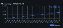
Ouch. One of my post-processing scripts, the one that creates a gigantic csv file, was "Killed" by Docker. That was the only message from Docker. No explanation, no logs, just "Killed".

Turned out there's a default 8GB memory limit per container and my script was terminated simply because it consumed more. I changed the setting to 16GB (maximum) - I hope it's enough :rolleyes:
docker-memory-stats.png

Edit: It was enough. Today's statistics updated. Data clean-up shows as more balanced numbers: tiles and catalogs are both at 3,013. Xmatch is bit behind: it's due to the out-of-coverage challenge I mentioned earlier. The "final no optical counterparts" have of course increased now that there are 59M detections in total, but the percentage remains the same, 0.09%.

Adding NeoWISE cross-match will decrease the number of suspected transients heavily. I think it's time to start working on that.
1766256073678.png
 
Last edited:
Ouch. One of my post-processing scripts, the one that creates a gigantic csv file, was "Killed" by Docker. That was the only message from Docker. No explanation, no logs, just "Killed".

Turned out there's a default 8GB memory limit per container and my script was terminated simply because it consumed more. I changed the setting to 16GB (maximum) - I hope it's enough :rolleyes:
View attachment 87250

Edit: It was enough. Today's statistics updated. Data clean-up shows as more balanced numbers: tiles and catalogs are both at 3,013. Xmatch is bit behind: it's due to the out-of-coverage challenge I mentioned earlier. The "final no optical counterparts" have of course increased now that there are 59M detections in total, but the percentage remains the same, 0.09%.

Adding NeoWISE cross-match will decrease the number of suspected transients heavily. I think it's time to start working on that.
New day and more challenges solved. No more huge CSV files: I switched to Parquet format. Size of master catalog decreased dramatically. Yesterday's 8GB memory requirement for a single script should not be a problem anymore.

I also made further improvements to the downloader. No file that is not 100% valid POSS-I red image will be taken to tiles-folder. Possible errors or weird situations with STScI service will be logged for possible inspection. This helps to keep the dataset clean, and possible backfills or other cross-tile actions will be much faster.

SExtractor caused a major headache: after few hours of debugging, I figured out it was creating quite large diagnostic files and left them in the data-folder. This behaviour is not documented anywhere. So I made a helper script that can be used to safely remove those files. They take quite a lot of disk space when you have downloaded thousands of tiles, and they are absolutely not needed.

Check the readme: https://github.com/jannefi/vasco?tab=readme-ov-file, make sure you downloaded/cloned the latest version, and remember to rebuild your docker image.

I used several hours to make this MOC plot o_O I didn't realise how difficult it can be to make this kind of simple image with Python. It should be easy, but for some reason many Python libraries had to be installed, upgraded, removed, downgraded, re-installed - and finally I ended up rewriting the whole script couple of times. But I finally won this battle against my machine: here's the coverage MOC of my tiles.

1766336240046.png
 
New day and more challenges solved. No more huge CSV files: I switched to Parquet format. Size of master catalog decreased dramatically. Yesterday's 8GB memory requirement for a single script should not be a problem anymore.

I also made further improvements to the downloader. No file that is not 100% valid POSS-I red image will be taken to tiles-folder. Possible errors or weird situations with STScI service will be logged for possible inspection. This helps to keep the dataset clean, and possible backfills or other cross-tile actions will be much faster.
Latest sw update :rolleyes:
The following MNRAS 2022 filters are now wired in:
- Pre‑xmatch filtering (FLAGS==0, SNR_WIN>30) and FWHM/elongation/SPREAD_MODEL
- Bright‑star/diffraction spike removal
- Gaia high‑proper‑motion check

This change requires going through all derived data if it has been processed (pipeline steps 2-5), but there's a simple script for that. More info here: https://github.com/jannefi/vasco/?tab=readme-ov-file#recent-improvements

The filtering is quite effective. Example of tile report (RA 121.001, DEC +41.736). This change will drop a lot of artefacts:

1766504692417.png
 
Last edited:
NEOWISE day has arrived :cool: This is a non-breaking and optional feature as usual, but important if you want to reproduce MNRAS 2022 and later publications. Main documentation updates in the workflow : https://github.com/jannefi/vasco/blob/main/WORKFLOW.md

Usual notes: always use the latest version of the sw, check the repo frequently. Remember to rebuild your docker container. I was too lazy to create actual versioned releases. Main-branch always contains the latest version, and it has been tested with at least a small amount of tiles. In any case, there's nothing harmful or risky with this sw. It just consumes a lot of disk space, but you can always delete the data.

This was a difficult feature to implement. NEOWISE-R Single Exposure (L1b) Source Table is a monster. I tried many different approaches on how to access and use the data as efficiently as possible. I ended up using TAP async jobs. I have to convert the data to VO tables (aka VOT) before passing them to TAP async calls with ADQL instructions (similar to SQL queries). This will require a) disk space although the VOT's can be deleted later on b) time -> TAP async calls can be slow. I had to be extra careful and submit data in smaller chunks. Otherwise IRSA often refuses to play. But with this approach, I can use multiple threads so that the data processing won't take days or weeks.

I have tested this feature only with a small subset of data, and it seems to work. Now the scripts are working on my full dataset (some 5000 30x30 arcmin tiles). It will take some hours to complete. All new data and statistics needs to be carefully analyzed. Hopefully after all this, I will be able to say that my dataset is close to MNRAS 2022 results. If results are not close enough, then I have some more checking todo.

Note that 2TB dedicated SSD won't be enough for full - or even 20-25% coverage - repro. I'm moving my pipeline from laptop to an environment that can scale and run 24x7 sometime during January-February. I managed to keep a fairly low budget, but the new environment is of course not free. But I wanted to continue this work and simply decided to invest bit more into this hobby.
 
Last edited:
This was a difficult feature to implement. NEOWISE-R Single Exposure (L1b) Source Table is a monster. I tried many different approaches on how to access and use the data as efficiently as possible.
Note and perhaps a question: it's quite possible all NeoWISE data can be accessed via AWS. See: https://registry.opendata.aws/wise-neowiser/

I was not able to make it work, though. I will have to try again because this approach would fully eliminate the need to make any external service calls. Data apparently sits there in Parquet format. It's comparable to all local setup where you have the full catalog stored on your computer.

Also see: https://nasa-irsa-wise.s3.us-west-2.amazonaws.com/index.html - data is obviously there o_O
 
Note and perhaps a question: it's quite possible all NeoWISE data can be accessed via AWS. See: https://registry.opendata.aws/wise-neowiser/

I was not able to make it work, though. I will have to try again because this approach would fully eliminate the need to make any external service calls. Data apparently sits there in Parquet format. It's comparable to all local setup where you have the full catalog stored on your computer.
Now the AWS version of Neowise "filtering" might actually work. It's not fully documented or tested, see: https://github.com/jannefi/vasco/pull/19 but there are now couple of new scripts that could be used to do the Neowise post-processing step. It just doesn't seem to be a good option for me: this huge dataset sits on AWS us-west-2. Due to the way this data is stored, the script needs to go through all of it, and the network becomes a bottleneck for me. I'm located in Finland using "average" network connection (max 100/100Mbs). In Finland, many people have much faster optical connections, hence the "average". I don't know the actual network connection statistics, though.

Anyone closer to us-west-2 or with a very fast connection to USA, may benefit from this approach so I decided to publish the scripts. They are self-explanatory - just look at the Makefile and think that these scripts can replace post-process steps 1.5/2 (make post15_sidecar) and 1.5/3 (Global QC summary). See the workflow: https://github.com/jannefi/vasco/blob/main/WORKFLOW.md Instead of TAPing Neowise, script reads data from AWS directly and does comparison locally. Note: because this takes so much time from Finland, I have not ran the script against all years (1-11 + addendum), and probably never will. If you want to try it, I suggest running it one year at a time using 8 threads. That can be much faster compared to "TAPping", but I just don't know. If you find any problem with the script, please post an issue ticket on github.
Caution: neowise_s3_sidecar.py will consume more RAM and CPU compared to the other scripts. Disk consumption depends on your dataset size. It creates Parquet "sidecar", which can be removed after reports are done. Also, these script won't run using the provided Docker image. It would need additional Python modules. I didn't list them, sorry. It's not a very difficult task, but I don't want to add them to the current Dockerfile in case only few people want to try.

There are possibly much faster options, but none of them are free. I considered trying AWS Athena https://aws.amazon.com/athena/?nc=sn&loc=1 because you could run all required queries in us-west-2 - this could be the fastest approach - and just download the results.

External Quote:
You are charged standard S3 rates for storage, requests, and data transfer. By default, query results are stored in an S3 bucket of your choice and are also billed at standard S3 rates.
With current S3 rates, and some well-thought query optimizations, I think it could cost less than 30$ + VAT (for one full run). Don't trust my estimates, though. Currently I'm not planning to pay for this service, because I often want to run all post-process steps to analyze current situation against MNRAS 2022 results. But again, this might be good to know in case you want to invest some money to get the Neowise results fast. If you want to try Athena-approach, do some good queries against year 8 of Neowise data first. If the cost is relatively slow, repeat the process for years 1-7, 9-11 and addendum. Addendum is quite small compared to others, so it might not be necessary.

Neowise is a monster: over 150 billion detections in total. It's by far the biggest catalogue used by this software. But it seems most of us, including me, are stuck with "TAPping". It's slow and gets slower when your dataset grows, but it works.

If anyone has any other ideas on how to tackle Neowise catalog faster with minimum cost, please leave a comment. I've spent several days with this one small part of software that just happens to take majority of the total processing time.
 
Sorry if they was covered before, but what are the dots with negative elevation?
Perhaps you mixed up declination with altitude? Negative values on this MOC are negative declinations. I probably should add Declination (°) label next to the y‑tick labels.

On this Mollweide-Aitoff‑style map the vertical axis is declination (−90° to +90°). Values below 0° are south of the celestial equator. This is my first MOC plot so it may look bit off.
 
Wow, it's 2026. Time for a new release :cool: the need to improve the software came again from user experience. My user experience :p.

I moved all my data to a 8-12TB disk that uses NTFS. I would not choose this filesystem, but I can't really complain or change it. This is my new environment, and the laptop didn't scale. But with this disk, the scripts started to slow down a lot during file and directory operations. NTFS is not designed to handle this kind of use case where we have thousands or 10s of thousands of folders - and lots of file operations happening on those folders.

So I introduced a "sharded" tree. Basically it looks like this: data/tiles_by_sky/ra_bin=*/dec_bin=*/tile-*` with 5° bins by default - lots of folders, but no folder is full of thousands of sub-folders. I used the same approach with Parquet data folders. NTFS is happy. Performance and reliability with NTFS and several other filesystems will improve due to this optional and non-breaking feature. More details here: https://github.com/jannefi/vasco?tab=readme-ov-file#directory-layout-and-sharded-tree

You can move your old data to the new sharded tree with one script: ./scripts/migrate_tiles_to_sharded.py. It takes two arguments: 1) --max-tiles - use this to limit of tiles for a run if you like. Useful if you have thousands of folders on a slow drive. 2) --go - optional, but the script doesn't start moving folders from old structure to the new one before you say --go.

I tried to change all downstream and helper scripts so that they will accept both folder structures and autodetect the new "tiles_by_sky" folder. I tested the scripts with a small 10 tile dataset so they should work, but you know what to do if they don't.
 
I have some good news and bad news. Get the latest version - all files - from github: https://github.com/jannefi/vasco/

Let's start with bad news. I found two bugs in the implementation (and configuration) of algorithms described in MNRAS 2022. The bug was minor, affecting the so called "spikes's removal" function. This fix alone would not be such bad news, it was just due to lazy unit testing. One that brings us to bad news was a configuration mistake in morphology filters. The algorithm reads output from a table produced by SExtracor (source extractor) and applies filtering based on various table values. Paper talks about additional filtering conditions. See the screenshot.
 mnras-2022-additional-algorithm.jpg


It's a fairly clear and not that difficult to implement. It would be really nice to have access to reference implementations of all algorithms. I'm sure all algorithms in MNRAS 2022 have been implemented by scientists many times. They are all common algorithms, but I couldn't find reliable and well tested reference implementations. Back to the issue: this was a stupid configuration mistake. SExtractor has very badly documented configuration files and it's easy to get things wrong with this critically important software. In this case I forgot to add several column names the algorithms expects: SPREAD_MODEL, SPREADERR_MODEL, XMAX-XMIN, YMAX-YMIN, XMAX-XMIN and YMAX-YMIN.

Algorithm cannot work as intended if it doesn't have values in these columns. In the worst case, when some value is absent, it is treated as 0. This could filter out all valid stars or galaxies from one tile, producing zero sources. It didn't happen for all tiles, but when it did, the software crashed and logged the error. Through log analysis, I noticed 18 "zeroed tiles" in my dataset (about 8,000 tiles). It took some time to figure out what the problem was. I thought it was a minor issue, because it only affected 18 tiles. But because the issue affects one key algorithm at the beginning of the pipeline, it is recommended to run steps 2-6, and all post-processing steps for all data (that has passed the pipeline). Otherwise data is not fully comparable to MNRAS 2022. I don't know yet how much this issue affects the final results: I'm now re-running my data through steps 2-6, and later on, through the post-pipeline steps. This will take some time. Re-running your dataset through the pipeline is the safest choice anyway. I made some helper script for clean-up and added instructions to release notes: https://github.com/jannefi/vasco/blob/main/RELEASE_NOTES.md

Note: you can run steps 2,3 using some parallelisation method. I'm now running with eight concurrent workers. After that, same applies to rest of the steps. I haven't documented parallel running of the basic steps yet. There are several ways of doing it. If you know Linux well enough, then you probably already know how to do this. If not, leave a note and I'll try to find some time to document a portable and reliable parallel running method.

I'm sure many astronomers/astrophysicists would have spotted these issues. It would be great if some person with matching skillset could review my code. I have tried to avoid implementing any astronomy/photometry algorithms and prefer offloading all "science math" tasks to software like psfex, SExtractor and stilts.

Good news: a lot of improvements and some possibly interesting helper scripts are available. Check the release notes for details. I made two plotters: one that shows your tile's location on full plate, and another one showing all plates with your tiles. It's interesting to see how close to plate edge some of the data might be, how much overlapping there is etc. After seeing one highly "populated" plate with 40+ tiles partially overlapping, I created "overlap aware randomised downloader". This is optional, so you need to give at least one additional parameter to the downloader. Again, check the release notes.

Here's one example of the full plate image. This is plate XE325 (some of you might be familiar with it already :), and my matching tiles. Note: I didn't attempt to implement full astrometrical calibration. Tile locations are approximately correct, based on the information available from FITS headers (PLATERA/PLATEDEC + PLTSCALE + X/YPIXELSZ for plate-level geometry). If you compare your tile locations with real astro-sw like Aladin, you will see the difference. More accurate plate polynomial can be added later if needed, but for now this pixel-math is sufficient (and fast).

dss1red_XE325.fits.png
 
Last edited:
Short update: I've implemented all missing checks except one: a Spanish Virtual Observatory (VOSA) specific query that I just couldn't figure out. But the impact of that query is small, so I'll just mark it as not done. I haven't tested the new code with full dataset yet so I can't really integrate it fully. Code is mostly in the repository (PTF, SuperCOSMOS, SkyBot, VSX), but please treat it as tentative.

I'm stuck with NeoWISE. Because of the bug mentioned earlier, I must run all data through all steps again. And like I mentioned before, this particular NeoWISE dataset is a monster and slow to query. IRSA (https://irsa.ipac.caltech.edu/frontpage/) has experienced some technical issues, service breaks, lot of concurrent queries etc. It has been fully offline few times during the past month. My NeoWISE queue is 55% complete, but it has taken almost a month. I can't run and monitor the pipeline 24/7 either so this will take a lot of time to complete. Only after that I can properly test, execute and publish final post processing step 1.6. Which will also take time because it involves TAP and other queries using various 3rd party services. Luckily the catalogs are not as big as NeoWISE.

Technically the most difficult query was Palomar Transient Factory aka PTF. That's why there are three different versions of the query in the repository. It took a lot of time to figure out what was wrong with the query because the backend error messages didn't help much. Turned out that one column name in the uploaded data is reserved for something. Here's one of the scripts that renames the "NUMBER" column: https://github.com/jannefi/vasco/blob/main/scripts/fetch_ptf_objects_stilts.sh
 
Last edited:
@HoaxEye thanks for your updates.

Did you end up having any further communication with Dr Villarroel or anyone from the VASCO team after her reply to you on Dec 4?
We did exchange some e-mails in December. Villarroel introduced me to Enrique Solano. Solano knows the technical side of the pipeline and all software. He tentatively agreed to review my pipeline, at least the key parts. There has been no progress, but I understood he is busy.
I also wrote to Villarroel this month asking for technical help, mainly related to the new post-process step 1.6: dataset/table names, service locations etc. She has not replied yet.

I didn't expect any help to begin with. Now I have one technical contact and Villarroel might be able to help with some of my latest questions. I'm not asking for code or other currently non-public material, because that could ruin the whole idea of independent replication.
 
Update: I have now implemented and tested a full replacement for post-process step 1.5, NASA's IRSA TAP async that uses NEOWISE-R Single Exposure (L1b) Source Table (neowiser_p1bs_psd) - with more than 150 billion source detections. You can freely use the code, but this alternative is by design not free: it's based on AWS services. I don't have exact cost estimates yet, because building and testing this required about 20-30 hours of EC2 computing time at about 1 USD/hour rate. Storage cost was nothing compared to the computing costs. I used r7g.4xlarge (Graviton3), which is quite heavy, but in the future the right size is probably r7g.2xlarge. The price is approx. $0.71 to $0.87 / hour. 10G storage volume should be enough.

Based on my tests, the script can handle 1,000 rows of data, end-to-end, in about 30-33 minutes (this can be up to 70x faster compared to same IRSA TAP async job). There are many variables that may affect processing time. Number one is location: I chose AWS us-west-2, because that's where the data is. See: https://registry.opendata.aws/wise-neowiser/ This is crucially important. The closer you can get to the data, the faster the whole process is. Data transfers to-from AWS using S3 takes some time, but it seems quite fast and very reliable. Again: if you want to try this approach, make sure all your AWS instances, storage etc. are located in us-west-2.

The goal of the architecture is to eliminate the performance issues, instability, and package loss inherent in large TAP async‑based queries at IRSA. The system accepts same csv-files that are already prepared for NASA's IRSA TAP async queries. So instead of TAP async, you send the same data via S3 to EC2 instance.

The "sidecar" that does the heavy duty work is here: https://github.com/jannefi/vasco/blob/main/scripts/neowise_s3_sidecar.py Now it has been tested with about 20 million rows of data that has previously passed IRSA TAP async service. Agreement rate is around 99.98%, which is good for this purpose. I can't explain the 0,02% difference, but I tried many different approaches and tweaks to reach 99.98%. NASA might be able to explain the difference. TAP async is basically a SQL server of sorts, so I think the data resides on a large database. In AWS, all data is stored in Parquet format. You have to build the query logic yourself. And it can be difficult and slow: if you read a "wrong" bin, you might have to wait for 20 minutes or hours (or run out of memory) because even the metadata can be huge.

I can't publish the detailed bash scripts that automate the data transfers, because they contain my personal AWS account and service identifiers. But it's not complicated: on your own PC/server, prepare and send all data to S3. On EC2, poll for data to appear on S3, then run it through the sidecar, convert results back to csv, push results to S3, delete all data from the instance, and wait for the next chunk. Repeat until done. Once you have all results stored safely on your PC or server, delete the EC2 instance, storage devices and S3. That way you can be assured there won't be any surprise costs. Just make sure you delete everything you created for this "neowiser pipeline".

If there is enough interest, I'll try to "anonymize" the 2-3 bash scripts that I'm using for automated data transfer. I tried to capture the basic idea in this picture.

AWS Neowiser - Architecture Overview.jpg


Edit: few additional things I forgot to mention
- With a large EC2 instance with many CPUs, you can use 16 parallel runners (or more). During development and testing, I used Graviton3. It handles 16 parallel runners nicely and performs well. Downsizing is a viable option and can drop costs, but the performance will suffer. I will do some trials with smaller EC2 instances along the way with smaller datasets, and post the results here.
- You can send bigger data chunks: I ended up using files with 1,000 rows because that's the default size for IRSA TAP queries. I can always switch back to IRSA if budget is tight, or when the data amount is small (e.g. hundred files). But I tested this setup with 200,000 rows files. It works, script can handle it if the EC2 instance has enough memory and computing power. But the overall performance does not necessarily improve much with larger files, it may actually suffer a bit. You might have to test with different chunk sizes to get optimal results, again depending on the selected EC2 instance and also size of storage. 200,000 rows fits easily on a 50G disk (that also contains the OS)
- I don't setup any extra services, including SSH. I have one script that installs the OS, Python, some tools and scripts, and starts the process. I connect to the instance using the AWS web-based Session Manager only when needed. It's clumsy and slow, but enough for setting up the environment and starting the pipeline.
- I also have a "teardown" script that deletes everything permanently: EC2, storage device, S3. Automating the full setup and teardown is important from cost perspective
- Monitoring is important: I made few monitoring scripts, but ended up using one on the pipeline PC (aka PROD/production), reading log files and S3 "queues". AWS monitoring tools are important if you up/downscale and perform tests with different instances, parallel runners, larger chunk files etc.
 
Last edited:
I can't publish the detailed bash scripts that automate the data transfers, because they contain my personal AWS account and service identifiers
Can't you just use environment variables and keep your bash scripts free of AWS creds?
[edit: actually, in hindsight, you probably know this already, but like m,e you've just taken the path of least resistance in an already complex process, just ignore me]
 
Can't you just use environment variables and keep your bash scripts free of AWS creds?
[edit: actually, in hindsight, you probably know this already, but like m,e you've just taken the path of least resistance in an already complex process, just ignore me]
That's exactly right: I took the path of least resistance :p

Time is literally money on AWS. Every hour spent on development and testing costs. Although the logic of pull/push scripts is simple, the implementation is hundreds of lines of bash-code. I implemented and tested them as fast as possible.

I'll try to improve the scripts during next runs. I don't want to publish untested scripts. There are also some missing tweaks like how to to deal with expiring AWS client sessions: I have no idea how to do that correctly with different types of accounts and login types.
 
I'll try to improve the scripts during next runs. I don't want to publish untested scripts. There are also some missing tweaks like how to to deal with expiring AWS client sessions: I have no idea how to do that correctly with different types of accounts and login types.
If you're wanting a hand, then I'd be happy to contribute. Just DM me if so.
 
Can't you just use environment variables and keep your bash scripts free of AWS creds?
[edit: actually, in hindsight, you probably know this already, but like m,e you've just taken the path of least resistance in an already complex process, just ignore me]
KISS:
Code:
phil@dovespaz:~$ cat awsauth
account=foobar
passwd = bazquux

phil@dovespaz:~$ AWS_AC=$(sed -n -e 's/^account\s*=\s*\(.*\)/\1/p' < awsauth);
phil@dovespaz:~$ echo $AWS_AC
foobar

phil@dovespaz:~$ AWS_PASSWD=$(sed -n -e 's/^passwd\s*=\s*\(.*\)/\1/p' < awsauth);
phil@dovespaz:~$ echo $AWS_PASSWD
bazquux
 
For anyone interested there has been a paper published to Arxiv on Feb 4, 2026 critical of the VASCO POSS-1 Transients:

Critical Evaluation of Studies Alleging Evidence for Technosignatures
in the POSS1-E Photographic Plates
by Wesley A Watters, et al

Dr Villarroel had this to say on twitter regarding the paper:
External Quote:
The samples they used contain positions but no timestamps. Without knowing exactly the time and date for any transient, that makes Earth's shadow tests and temporal correlations shaky, and the guesswork in Section 4.1. introduces huge uncertainties. Combined with aggressive filtering, this inevitably affects statistical power and introduces bias. The shadow deficit is not expected to be seen above a 1.7 sigma level with 5000 objects only.
Also here is an AI generated rebuttal of this new paper courtesy of the Good Trouble Show
I suspect this post should be in the other thread -- https://www.metabunk.org/threads/transients-in-the-palomar-observatory-sky-survey.14362/ -- since this one is for recreating the results.
 
I suspect this post should be in the other thread -- https://www.metabunk.org/threads/transients-in-the-palomar-observatory-sky-survey.14362/ -- since this one is for recreating the results.

Thanks. I want through the Watters et al. pre-print. Sigh. Good points, but this means more work, too.

My pipeline keeps record of plate IDs, and all relevant info from full plate headers, which are now published in the repository. This is true for all detections. Early on it was easy to see that public MNRAS 2022 datasets do not include this information so I added them. I recently made a design decision to write the DSS plate identifier also in Parquet format (for downstream consumers), and it has been implemented. This is because some downstream consumers will need plate-level epoch.

In addition to external catalog gates and cross-scan comparisons (implemented, but not yet ran with full dataset), I must add a secondary HPM sweep and a light symmetry/PSF residual check. Result should be "R_like", meaning "set R" discussed in Watters et. al.

Also, I probably must produce per‑plate 2‑D density maps. And normalize all temporal analyses to actual observing days. And most likely run against NEOWISE with varying parameters, not just one like now. Hoping all this helps when it comes to analyzing my dataset. My todo-list just already feels endless with many time consuming tasks. The missing external catalog runs have a top priority, so these possible new work items must wait.

I'm not going to speculate what Watters et. al. paper means in detail. Just observing:

For object level (a starlike object), nothing changes. It will remain - even if I one day publish meaningful results - a "Schrödinger issue" (referring to earlier critique by Hambly & Blair). Both claims can be true: any source can be mundane (emulsion issue, plate defect, scan problem) or astrophysical (a true short‑duration optical flash). Only microscopy can decisively choose. I don't see any other way.

For the population‑level (plates & tiles & datasets etc.) claims challenged by Watters et. al.: no microscopy is required to show prior analyses were not robust. I'll try to improve the replication effort so this dataset won't face similar criticism The list of required actions is not necessarily exhaustive or accurate. I haven't even planned implementing Earth's shadow calculations or any other item from 2025 papers. I need to finish MNRAS 2022 first.

I'm not trying to reproduce any ET UFO claims. Those are just hypothesis. This was supposed to be a simple pipeline replication. Except it's far from simple.

Edit: I decided to publish "interpretation policy" document: https://github.com/jannefi/vasco/blob/main/docs/Interpretation_policy.md
 
Last edited:
Also here is an AI generated rebuttal of this new paper courtesy of the Good Trouble Show

I read the Good Trouble Show article. It's an excellent example of how not to use LLM AIs for scientific analysis. There are two fair or "OKish" points made by AIs in this article, but the rest is totally unreliable. To the extent that even the OKish points are worthless.

Author says an extra private critique was given to the AIs, but that was not shared with the readers. That's called prompt steering. I hope they didn't do this deliberately.

All prompts and AI input files should have been disclosed. If we don't know all the inputs, the outputs can be basically anything. This approach is unverifiable and unreliable.

Cross-feeding model outputs to each other to form "consensus" might feel rigorous, but it is actually "groupthink via prompt‑chaining". If each round seeds the next with highlighted "fatal flaws," you amplify earlier biases. You can use several AIs to cross-check topics, but not like this. Again, we would need to see the prompts and input files. All of them.

Author lists just one 2025 Villarroel paper (the aligned, multiple‑transient events paper) and the Watters critique. There is no mention of the 2025 "image profiles" paper which specifically addresses the "narrower FWHM" debate the Substack spends time on. This sounds like omission of relevant analysis information (but they did feed undisclosed extra, private critique). At least currently, you must give all relevant input files, not just snippets or conclusions to an AI tasked to perform scientific analysis. Otherwise LLMs tend to use a fallback method: web search that usually feeds irrelevant data when we talk about scientific publications/analysis.

You can use AIs to help with scientific analysis, but you need to know how to do it properly and transparently. Otherwise your "rebuttal" or "debunk" is worth nothing.
 
Milestone in my POSS‑I / VASCO replication project. All MNRAS‑compatible filters from Solano+Villarroel+Rodrigo (2022) are now implemented in my open‑source pipeline (two‑pass SExtractor/PSFEx, morphology gates, USNO‑B spike rules, Gaia/PS1/IR/SCOS checks, Skybot, etc).

First preliminary survivors are now produced — a small set of candidates that pass all gates. See: https://github.com/jannefi/vasco/wiki/Overview for details

I also published the 150 candidates: https://github.com/jannefi/vasco/blob/main/metadata/survivor_set_150_rows_1502-2026.csv

Despite all the efforts put into software and methods, the final survivors obtained from my dataset (~150 objects across ~8,100 POSS‑I tiles) show zero positional overlap with the S=298,165 or R=5,399 survivors published by MNRAS 2022, with nearest separations of ~1.4 degrees.

This mismatch is expected because the MNRAS upstream dataset (their unpublished "A" set):

- maybe subject to undocumented pre‑filtering,
- apparently missing ~300 POSS plates (according to Watters et al. 2026)
- perhaps shaped by manufacturing, scanning, and emulsion defects,
- possibly dominated by plate-edge and artifact clustering,
- and does not reflect an actual astronomical distribution, according to Watters et al. (2026)

Work continues. I still need a lot more data. And all that data needs to go through the full pipeline and post-processing steps. But now all "filtering" should be in place, so I'll just keep collecting tiles and let the pipeline do the work.

I would love to publish all my data, but it's currently over 2TB. I have no place where I could publish that amount of data (without paying for storage). If I manage to reach 20-25% of POSS-I coverage, all data will probably take about 7-10TB disk space.
 
I would love to publish all my data, but it's currently over 2TB. I have no place where I could publish that amount of data (without paying for storage). If I manage to reach 20-25% of POSS-I coverage, all data will probably take about 7-10TB disk space.
According to this HuggingFace "usually" offers up to 5TB of free public storage, although it's a bit unclear as the free limits are subject to whether it is deemed to be "impactful work". Maybe you could look for an even better lossless compression of the input data ?
 
Last edited:
Back
Top